Download this tutorial as a Jupyter notebook
Discover Cost-Efficient AI Customer Service Agents with NVIDIA Data Flywheel Blueprint#

This notebook demonstrates the end-to-end process of using the Data Flywheel Blueprint to continuously identify and promote more cost-efficient agents for an AI-powered customer service assistant.
Data Flywheel Blueprint#
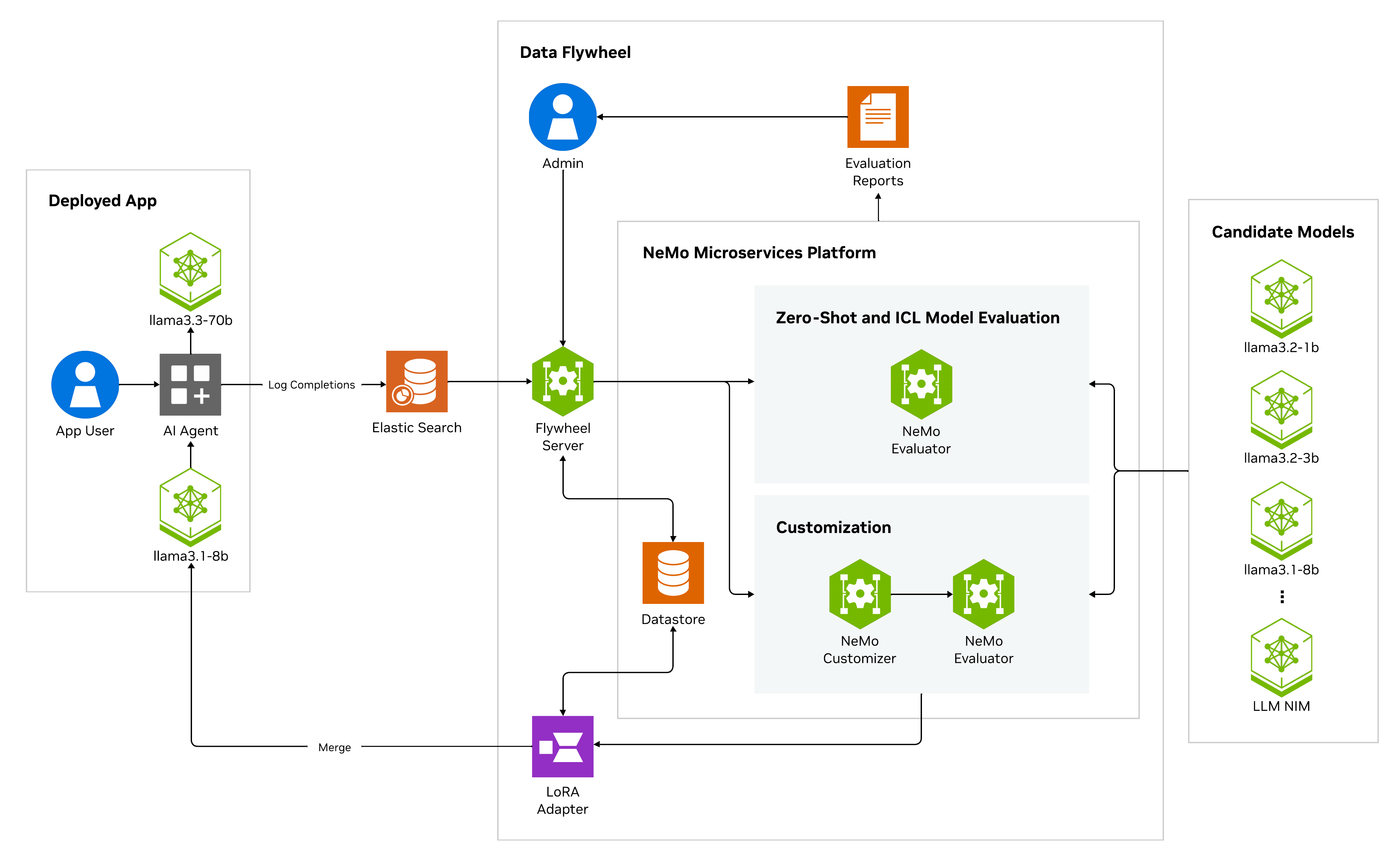
The NVIDIA Data Flywheel Blueprint provides a systematic, automated solution to refine and redeploy optimized models that maintain accuracy targets while lowering resource demands. This blueprint establishes a self-reinforcing data flywheel, using production traffic logs and institutional knowledge to continuously improve model efficiency and accuracy.
AI Virtual Assistant for Customer Service#
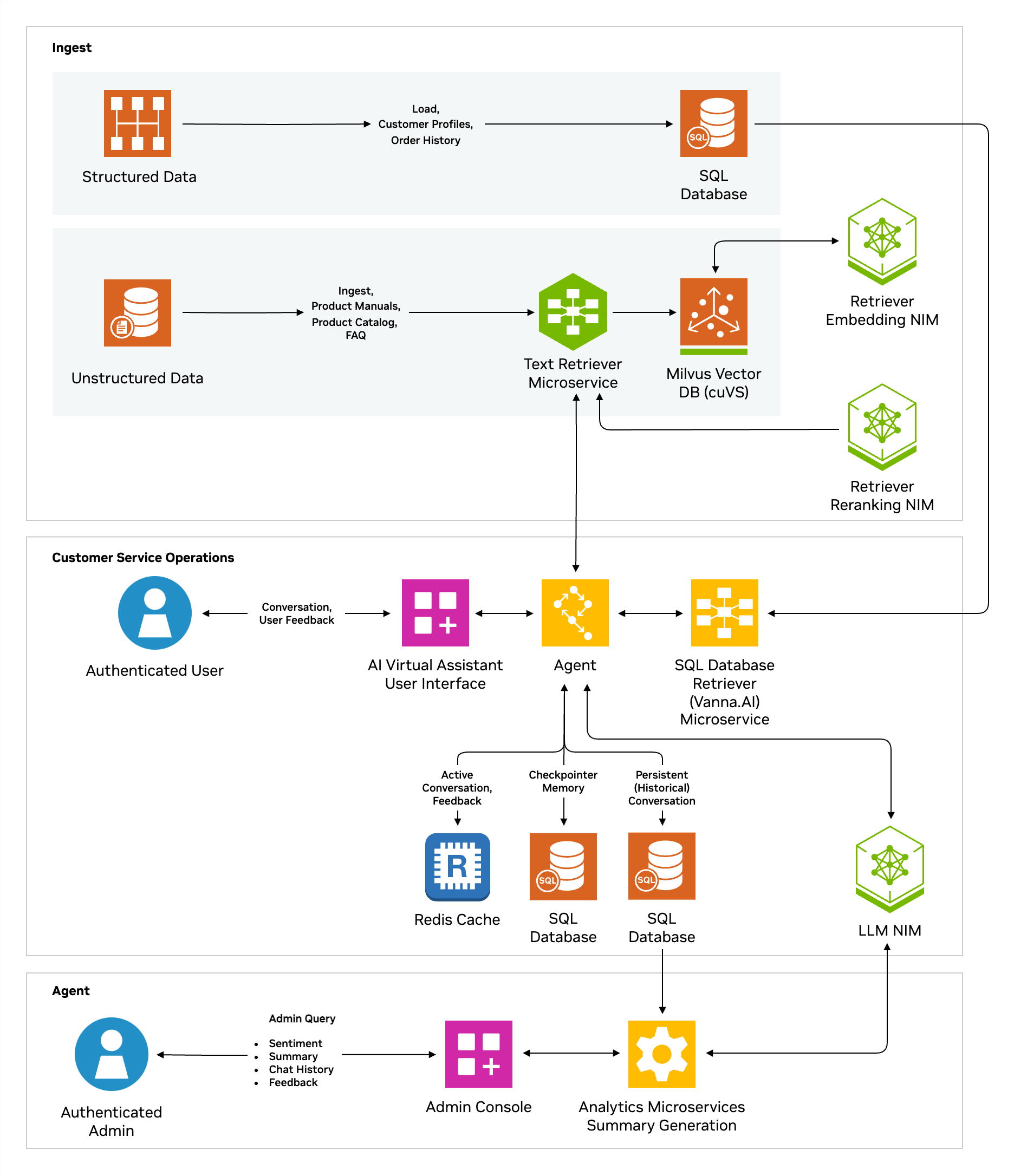
The AI virtual assistant (AIVA) for customer service NIM Agent Blueprint, powered by NVIDIA NeMo Retriever™ and NVIDIA NIM™ microservices, along with retrieval-augmented generation (RAG), offers a streamlined solution for enhancing customer support. It enables context-aware, multi-turn conversations, providing general and personalized Q&A responses based on structured and unstructured data, such as order history and product details.
AIVA employs a multi-agent architecture, where each user query is processed through multiple specialized agents, requiring several LLM calls per interaction. While this design ensures accuracy, it also introduces high latency, especially when using large models like Llama-3.3-70B or Llama-3.1-Nemotron-Ultra-253B-v1, potentially impacting user experience.
To mitigate this, we leverage the Data Flywheel Blueprint to distill smaller models that maintain comparable accuracy to larger ones. By utilizing production traffic from AIVA, this approach significantly reduces response latency while preserving model quality and reliability.
Contents#
1. Data Flywheel Blueprint Setup#
Step 1: Set NGC API key following the instructions at Generating NGC API Keys.
import os
from getpass import getpass

os.environ['NGC_API_KEY'] = getpass("Enter your NGC API Key")
Step 2: Clone the data flywheel repo and fetch data files.
This step presents two options:
Step 2 (Option 1) NVIDIA Brev Launchable Setup: The instructions below apply only to users running this notebook via the Brev Launchable.
NVIDIA Brev is a developer-friendly platform that makes it easy to run, train, and deploy ML models on cloud GPUs without the hassle of setup—it comes preloaded with Python, CUDA, and Docker so you can get started fast.
%%bash
git clone https://github.com/NVIDIA-AI-Blueprints/data-flywheel.git
cd data-flywheel
sudo apt-get update && sudo apt-get install -y git-lfs
git lfs install
git-lfs pull
import sys
from pathlib import Path

notebook_dir = Path.cwd()
project_root = notebook_dir / "data-flywheel"
data_dir = project_root / "data"
sys.path.insert(0, str(project_root))
os.chdir(project_root)
print(f"Working directory changed to: {Path.cwd()}")
Step 2 (Option 2) Self-Hosted Notebook Setup: The instructions below apply only to users running this notebook on their own setup (i.e., if you followed the pre-requisites in the Data-Flywheel Blueprint Github README for hardware and software requirements, to clone the repo, and start Jupyter Notebook.)
Note: If you are using a Brev Launchable, please follow Option 1 above in this step.
## Important: Uncomment and run this cell in a self-hosted notebook setup

# from pathlib import Path

# notebook_dir = Path.cwd()
# project_root = notebook_dir.parent
Step 3: Install python dependencies
%%bash
cd ..
source .venv/bin/activate
python -m ensurepip --upgrade
python -m pip install --upgrade pip setuptools wheel
pip install elasticsearch==8.17.2 pandas>=2.2.3 matplotlib==3.10.3 pydantic==2.11.3 pydantic-settings==2.9.1 nemo-microservices==1.1.0
Step 4: Update config/config.yaml to use remote LLM as judge. By default, the Data Flywheel Blueprint deploys LLama-3.3-70B-instruct locally for LLM as a judge, which requires 4 GPUs. But for the launchable, we will choose the remote LLM judge and use the LLama-3.1-70B-instruct NIM hosted on build.nvidia.com. Feel free to skip this setp if you plan to use a local LLM as the judge.
For this notebook, we will use only meta/llama-3.2-1b-instruct, meta/llama-3.2-3b-instruct, and nvidia/llama-3.1-nemotron-nano-8b-v1 in the flywheel but you can uncomment other models in the yaml file to include in the flywheel run. You can also change other config settings such as data split and training hyperparameters as desired. Users can also disable model customization (fine-tuning) by setting customization_enabled to false.
For more details on the configuration for running data flywheel, please refer to Configuration Guide.
import re
from textwrap import dedent

config_path = project_root / "config" / "config.yaml"

new_llm_block = dedent("""\
llm_judge_config:
  deployment_type: "remote"
  url: "https://integrate.api.nvidia.com/v1/chat/completions"
  model_name: "meta/llama-3.1-70b-instruct"

""")

new_nims_block = dedent("""\
nims:
  - model_name: "meta/llama-3.2-1b-instruct"
    model_type: "llm"
    context_length: 8192
    gpus: 1
    pvc_size: 25Gi
    tag: "1.8.3"
    customization_enabled: true
    customizer_configs:
      target: "meta/llama-3.2-1b-instruct@2.0"
      gpus: 1
      max_seq_length: 8192

  - model_name: "meta/llama-3.2-3b-instruct"
    model_type: "llm"
    context_length: 8192
    gpus: 1
    pvc_size: 25Gi
    tag: "1.8.3"
    customization_enabled: true
    customizer_configs:
      target: "meta/llama-3.2-3b-instruct@2.0"
      gpus: 1
      max_seq_length: 8192

  - model_name: "meta/llama-3.1-8b-instruct"
    model_type: "llm"
    context_length: 8192
    gpus: 1
    pvc_size: 25Gi
    tag: "1.8.3"
    customization_enabled: true
    customizer_configs:
      target: "meta/llama-3.1-8b-instruct@2.0"
      gpus: 1
      max_seq_length: 8192

  # - model_name: "nvidia/llama-3.1-nemotron-nano-8b-v1"
  #   model_type: "llm"
  #   context_length: 4096
  #   gpus: 1
  #   pvc_size: 25Gi
  #   tag: "1.8.4"
  #   customization_enabled: true
  #   customizer_configs:
  #     target: "nvidia/nemotron-nano-llama-3.1-8b@1.0"
  #     gpus: 1
  #     max_seq_length: 4096

""")

text = config_path.read_text()

def replace_block(yaml_text: str, key: str, new_block: str) -> str:
    pattern = rf"(?ms)^({re.escape(key)}:[\s\S]*?)(?=^\S|\Z)"
    return re.sub(pattern, new_block, yaml_text)

text = replace_block(text, "llm_judge_config", new_llm_block)
text = replace_block(text, "nims", new_nims_block)

config_path.write_text(text)
print("config.yaml updated")
To use remote LLM as judge, we will set the API key to access the remote LLM. You can create an API Key at https://build.nvidia.com/settings/api-keys.
os.environ['NVIDIA_API_KEY'] = getpass("Enter your NVIDIA API Key")
Step 5: Start data flywheel service, which involves first deploying the Nemo Microservices and then bring up the data flywheel service via docker compose with MLFlow enabled. This step may take about 10 minutes.
Note: The
deploy-nmp.shscript automates the deployment of NeMo Microservices. For manual setup or advanced configuration, please consult the NeMo Microservices documentation.
If you choose to manually deploy the Nemo Microservices Platform, then make sure you update the nmp_config field in the config/config.yaml with the correct base urls. The default is:
nmp_config:
      nemo_base_url: "http://nemo.test"
      nim_base_url: "http://nim.test"
      datastore_base_url: "http://data-store.test"
%%bash
set -e

log() {
  echo -e "\033[1;32m[INFO]\033[0m $1"
}

echo "$NGC_API_KEY" | docker login nvcr.io -u '$oauthtoken' --password-stdin
chmod +x scripts/deploy-nmp.sh
./scripts/deploy-nmp.sh --progress
log "Starting data flywheel service..."
export COMPOSE_PROFILES=mlflow && docker compose -f deploy/docker-compose.yaml up -d --build >> flywheel_deploy.log 2>&1
log "Data flywheel service started successfully!"
2. AI Virtual Assistant Application Setup#
In this example, we’ll use AIVA as the reference application to illustrate how the Data Flywheel Blueprint can be leveraged to reduce inference latency. We start by deploying the AIVA application. To enable observability, the original AIVA implementation is wrapped with the NeMo Agent Toolkit, which provides a Data Flywheel plugin for seamlessly exporting runtime traces in the schema expected by the Data Flywheel Blueprint to its Elasticsearch instance.
For additional details on wrapping AIVA or other GenAI applications with the NeMo Agent Toolkit, see the NeMo Agent Toolkit documentation.
2.1 Deploy AIVA#
%%bash
# Clone repository
cd ..
git clone --branch nat-dfw-integration https://github.com/NVIDIA-AI-Blueprints/ai-virtual-assistant.git
cd ai-virtual-assistant

export APP_CHAT_LLM_MODELNAME=meta/llama-3.3-70b-instruct
# export APP_CHAT_LLM_SERVERURL=http://nim.test  ## uncomment if model deployed locally with NMP

export PRIMARY_ASSISTANT_LLM_MODELNAME=meta/llama-3.3-70b-instruct
# export PRIMARY_ASSISTANT_LLM_SERVERURL=http://nim.test  ## uncomment if model deployed locally with NMP

export ORDER_STATUS_LLM_MODELNAME=meta/llama-3.3-70b-instruct
# export ORDER_STATUS_LLM_SERVERURL=http://nim.test  ## uncomment if model deployed locally with NMP

export RETURN_PROCESSING_LLM_MODELNAME=meta/llama-3.3-70b-instruct
# export RETURN_PROCESSING_LLM_SERVERURL=http://nim.test  ## uncomment if model deployed locally with NMP

export APP_LLM_MODELENGINE=nvidia-ai-endpoints
export DATA_FLYWHEEL_CLIENT_ID=nat-ai-virtual-assistant
export DATA_FLYWHEEL_ENDPOINT=http://localhost:9200
export DATA_FLYWHEEL_ES_INDEX=flywheel

docker compose -f deploy/compose/docker-compose.nat.yaml up -d --build >> aiva_deploy.log 2>&1
docker compose -f src/ingest_service/docker-compose.yaml run --rm ingest-client >> aiva_deploy.log 2>&1
Note: deploying the full AIVA will application take roughly 10 to 20 mins.
2.2 Interact with AIVA and View Logs#
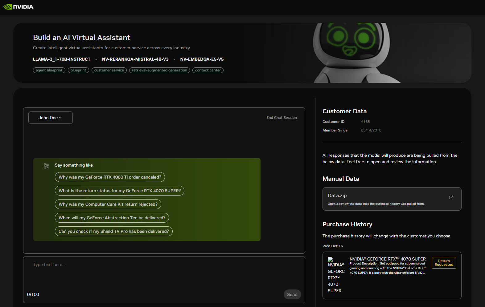
Next navigate to your Brev instance page, go to the Access tab, select Using Secure Links, find and click the link that looks like https://aiva-xxxxxx.brevlab.com which will take you the AIVA application UI(shown below).
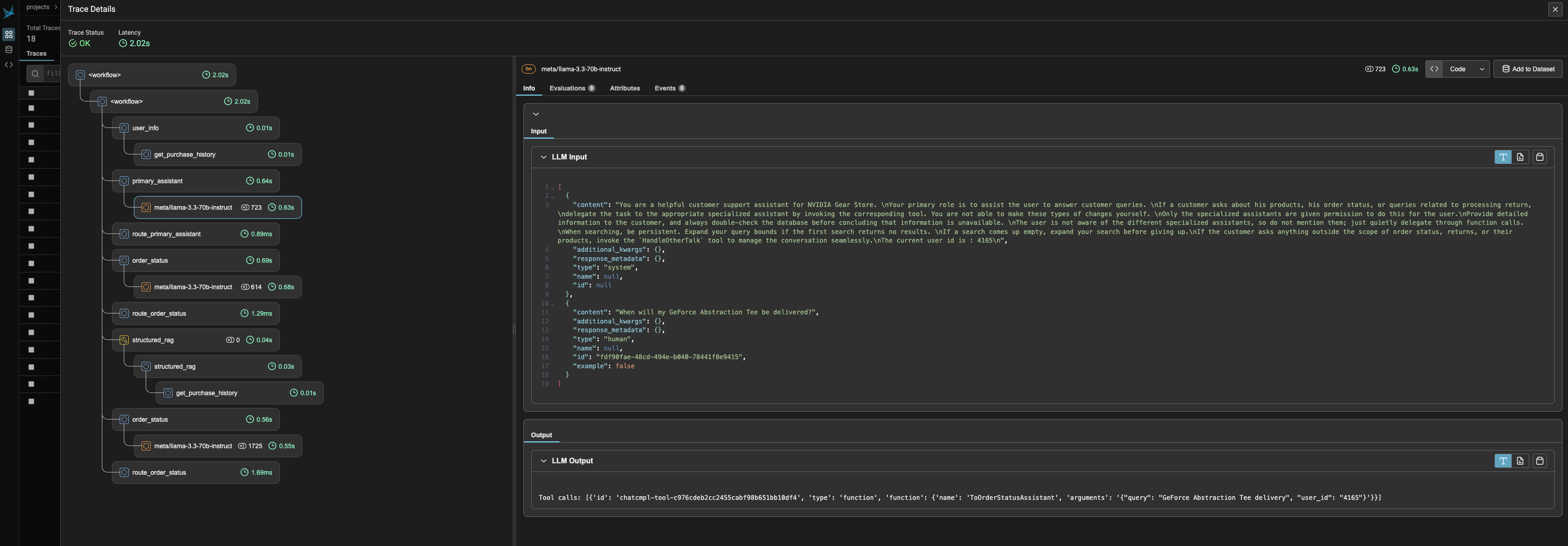
Below you will find the call graph for AIVA.
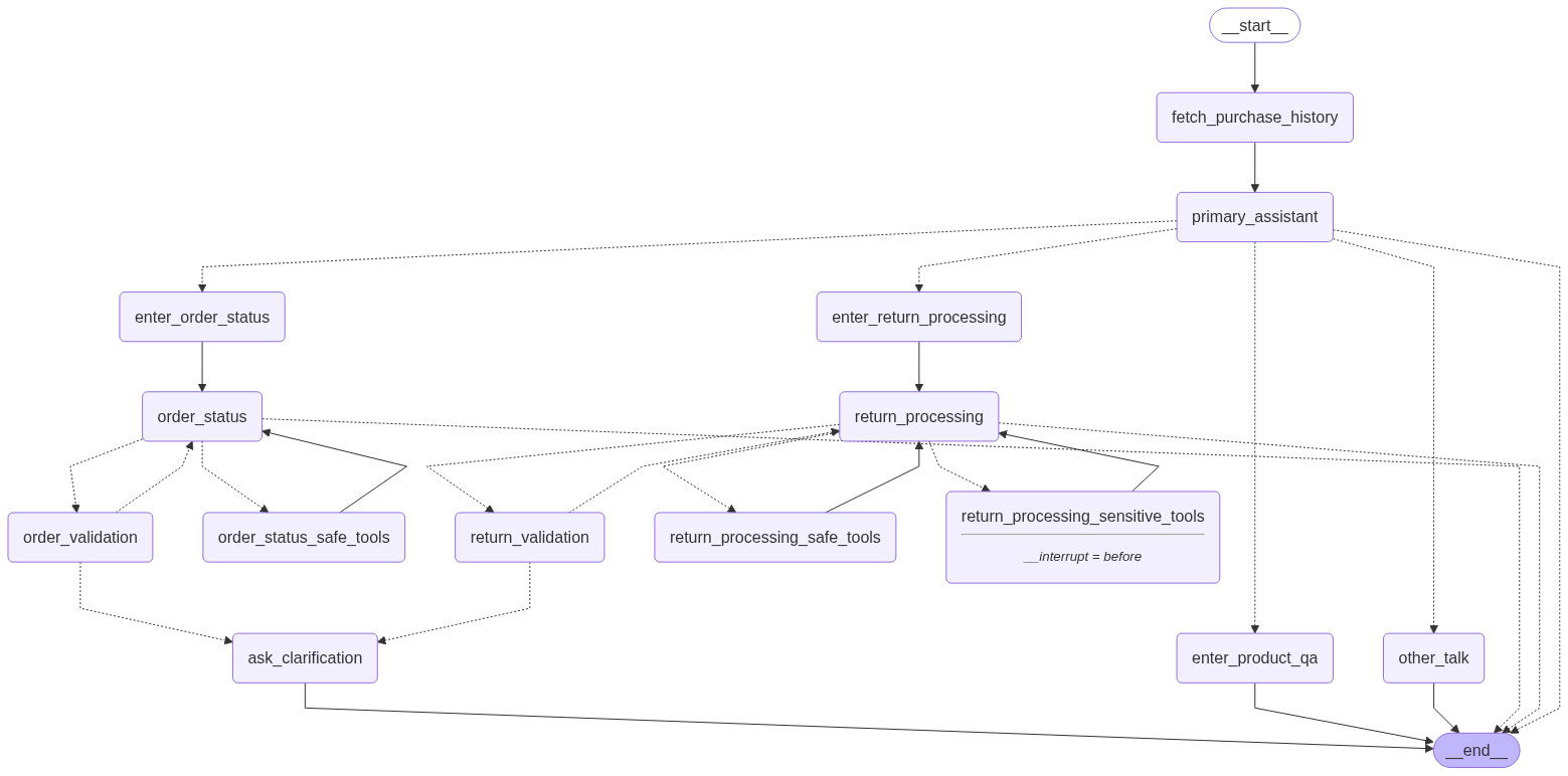
You can see that AIVA is a multi-agent application implemented with LangGraph, where each agent node (e.g., primary_assistant, order_status, return_processing, etc.) is wrapped with the NeMo Agent Toolkit’s @register_function decorator to enable observability and workload scoping. To learn how to migrate the original AIVA implementation to the NeMo Agent Toolkit and gain built-in observability and Data Flywheel capabilities, check out this guide.
The Data Flywheel Blueprint uses workload identifiers (workload_id) to organize traces for targeted model optimization. When AIVA is wrapped with the NeMo Agent Toolkit, each agent node functions as a registered component and automatically receives a workload_id corresponding to its function/node name. For example, LLM calls within the order_status agent are associated with the order_status workload unless a lower-level function containing the LLM call is wrapped again and defines its own scoped workload_id.
Default Scoping Behavior: By default, each trace inherits a workload_id from its parent NeMo Agent Toolkit registered function. The combination of client_id and workload_id is then used by the Data Flywheel to filter and select data for subsequent training jobs.
Feel free to use the example queries to interact with the application. Once a query completes, you can view the exported traces in the Elasticsearch index.
The following command retrieves the most recent logged schema:
%%bash
curl -s "http://localhost:9200/flywheel/_search?size=1&sort=timestamp:desc" | jq '.hits.hits[0]._source'
The NAT implementation of AIVA also comes with Phoenix observability plugin to help you better visualize the agent trace/trajectory. To use Phoenix, navigate to your Brev instance page, go to the Access tab, select Using Secure Links, find and click the link that looks like https://phx0-xxxxxxxx.brevlab.com which will take you the Phoenix UI (shown below).
3. Run a Flywheel Job#
3.1 Load Sample Dataset#
You can continue interacting with the AIVA application to generate logs for Flywheel, which helps drive meaningful improvements over the base candidate models. To speed up the process, we’ve also provided a sample set of pre-generated AIVA logs that you can load directly into Elasticsearch.
This sample was created by first generating synthetic user queries with NeMo Data Designer, then passing those queries into AIVA to produce logs. NeMo Data Designer is purpose-built for AI developers to create high-quality, domain-specific synthetic data at scale—unlike general-purpose LLMs that often struggle to deliver consistent and reliable results. You can start from scratch or use your own seed datasets to accelerate AI development with greater accuracy and performance. To learn how to generate synthetic user queries using NeMo Data Designer, check out the SDG notebook.
First, we need to import required libraries and configure pandas display options for better readability in notebook outputs.
import sys
from pathlib import Path
import requests
import time
from datetime import datetime
import json
import pandas as pd
from IPython.display import display, clear_output
import random

pd.set_option('display.max_columns', None)  # Show all columns
pd.set_option('display.width', None)        # Width of the display in characters
pd.set_option('display.max_colwidth', None)  # Show full content of each cell
Use the provided sample dataset from AI Virtual Assistant (aiva) (data/aiva_primary_assistant_dataset.jsonl) to simulate real user logs captured while an agentic customer service agent application is running. Each data point has the following schema:
Field |
Type |
Description |
|---|---|---|
|
|
Time the request was issued |
|
|
Stable identifier for the logical task / route / agent node |
|
|
Identifier of the application or deployment that generated traffic |
|
|
Exact |
|
|
Exact |
The request uses the OpenAI ChatCompletions request format and contains the following attributes:
modelincludes the Model ID used to generate the response.messagesincludes asystemmessage as well as auserquery.toolsincludes a list of functions and parameters available to the LLM to choose from, as well as their parameters and descriptions.
%%bash
DATA_PATH = data_dir / "aiva_primary_assistant_dataset.jsonl"

head -n1 {DATA_PATH} | jq
The data points generated by AI Virtual Assistant in response to user queries are considered ground truth.
Ground truth data points are used to evaluate and customize more efficient models that can perform similarly to the current model. This customization process is analogous to a student-teacher distillation setup, where synthetic data generated from the teacher model is used to fine-tune a student model.
Next, we’ll load the data into Elasticsearch using a helper method load_data_to_elasticsearch, making it accessible to the Data Flywheel service.
from src.scripts.load_test_data import load_data_to_elasticsearch

load_data_to_elasticsearch(file_path=DATA_PATH)
3.2 Launch Flywheel Job#
Initiate a Flywheel job by sending a POST request to the /jobs API. This triggers the workflow asynchronously.
In production environments, you can automate this process to run at scheduled intervals, in response to specific events, or on demand.
For this tutorial, we will target the primary customer service agent by setting the workload_id to “primary_assistant” and we will set client_id to “aiva-1” which has 300 data points.
# Flywheel Service URL
API_BASE_URL = "http://localhost:8000"

response = requests.post(
    f"{API_BASE_URL}/api/jobs",
    json={"workload_id": "primary_assistant", "client_id": "aiva-1"}
)

response.raise_for_status()
job_id = response.json()["id"]

print(f"Created job with ID: {job_id}")
For each candidate model, the data flywheel runs evaluations on the base model and its in-context learning (ICL) variant. If customization is enabled, the model is fine-tuned and evaluated again.
4. Monitor Job Status#
4.1 Check Job Status#
Submit a GET request to /jobs/{job_id} to retrieve the current status.
def get_job_status(job_id):
    """Get the current status of a job."""
    response = requests.get(f"{API_BASE_URL}/api/jobs/{job_id}")
    response.raise_for_status()
    return response.json()
get_job_status(job_id)
In the job status output, you will see the following metrics for evaluating the accuracy of tool calling once evaluations get completed:
Metric Name |
Definition |
Scoring Criteria |
Notes |
|---|---|---|---|
Function name accuracy |
Checks if the predicted function name exactly matches the ground truth function name. |
1 if predicted function name is an exact match; 0 otherwise. |
Evaluates only the function name, not arguments. |
Function name + args accuracy (exact-match) |
Checks if both the function name and all arguments exactly match the ground truth. |
1 if both function name and all arguments are exact matches; 0 otherwise. |
Strictest metric; all parts must match exactly. |
Function name + args accuracy (LLM-judge) |
Checks if the function name matches exactly, and arguments are either exact matches or semantically equivalent. |
1 if function name matches and each argument is either an exact match or semantically correct (as judged by an LLM); 0 otherwise. |
Allows semantic similarity for complex arguments; captures intent and functional correctness even with paraphrasing. |
To simplify the process and enable continuous monitoring, we defined a utility function monitor_job in utils/job_monitor_helper.py:
Periodically retrieve the job status
Format the output into a table
When any evaluations get completed, it fetches detailed results from the NeMo Evaluator Microservice, and uploads them to MLflow for visualization.
This makes it easier to compare and analyze the results.
(Optional) Viewing the MLflow dashboard#
If MLflow visualization is enabled, the MLflow dashboard will be available at port 5000 (default)
If using Brev Launchable: Navigate to your Brev instance page, go to the
Accesstab, selectUsing Secure Links, and click the link that looks likehttps://mlflow-*.brevlab.com. As evaluation jobs complete, they will be logged in MLflow with their flywheeljob_idas the MLflow experiment name.If using a Self-Hosted Notebook Setup: Open your browser and go to
<local-IP>:5000
4.2 Run Continuous Monitoring#
Note: The first customization run typically takes about 10 minutes to start while the training container is being downloaded. The
monitor_jobcall in the cell below usually requires around 50 minutes to complete training and evaluation of the candidate NIMs, though the exact duration may vary depending on the specific GPU and the responsiveness of the remote endpoint used for LLM-judge evaluations.As the evaluations complete, you will begin to see metrics appear in both the table and the MLflow dashboard.
from notebooks.utils.job_monitor_helper import monitor_job

monitor_job(
    api_base_url=API_BASE_URL,
    job_id=job_id,
    poll_interval=5
)
You’ve now successfully completed a Flywheel run and can review the evaluation results to decide whether to promote the customized or ICL model. However, with only 300 data points, the customized Llama-3.2-1B-instruct is likely still limited in accuracy.
That said, the Data Flywheel operates as a self-reinforcing cycle—models continue to improve as more user interaction logs are collected. Below, we demonstrate how the model accuracy improves incrementally with additional data.
5. Show Continuous Improvement (Optional)#
To extend the flywheel run with additional data, we’ll launch a new job using client_id set to “aiva-2”, which includes 500 data points, to evaluate the impact of increased data volume on performance.
Note that client_id is originally intended to identify the client that generated the traffic. However, in the notebook, it was repurposed to represent datasets of varying sizes, illustrating the progressive improvement of the data flywheel as more data is collected.
response = requests.post(
    f"{API_BASE_URL}/api/jobs",
    json={"workload_id": "primary_assistant", "client_id": "aiva-2"}
)

response.raise_for_status()
job_id = response.json()["id"]

print(f"Created job with ID: {job_id}")
monitor_job(
    api_base_url=API_BASE_URL,
    job_id=job_id,
    poll_interval=5
)
You should see some improvements of the customized model compared to the last run.
Assuming we have now collected even more data points, let’s kick off another flywheel run by setting client_id to “aiva-3” which includes 1,000 records.
response = requests.post(
    f"{API_BASE_URL}/api/jobs",
    json={"workload_id": "primary_assistant", "client_id": "aiva-3"}
)

response.raise_for_status()
job_id = response.json()["id"]

print(f"Created job with ID: {job_id}")
monitor_job(
    api_base_url=API_BASE_URL,
    job_id=job_id,
    poll_interval=5
)
After the run with 1,000 data points, we should observe the customized model’s accuracies improving significantly, with the Function name accuracy approaching 1.0.
This indicates that the customized LLama-3.2-1B-instruct model achieves accuracy comparable to the much larger LLama-3.3-70B-instruct base model deployed in AI Virtual Assistant, while significantly reducing latency and compute usage thanks to its smaller size.
In the next step, we will show how to deploy the customized LLama-3.2-1B-instruct and run inference with it.
6. Deploy Customized Model for Latency Reduction {#6}#
Now that we have a fine tuned smaller model that matches the accuracy of the larger model currently production, we can deploy the smaller model to replace the larger model in production.
To do this, we will leverage two component microservices from the NeMo Microsevices Platform to simplify model deployment and inference:
NeMo Deployment Management: Provides an API to deploy NIM on a Kubernetes cluster and manage them through the NIM Operator microservice.
NeMo NIM Proxy: Provides a unified endpoint that you can use to access all deployed NIM for inference tasks.
We will deploy the fine tuned LLama-3.2-1B-instruct model to replace the Primary Assistant LLM as an example. First, let’s deploy the base model:
6.1 Initialize Nemo Microservices Client#
from nemo_microservices import NeMoMicroservices

# Configure microservice host URLs
NEMO_BASE_URL = "http://nemo.test"
NIM_BASE_URL = "http://nim.test"

# Initialize the client
nemo_client = NeMoMicroservices(
    base_url=NEMO_BASE_URL,
    inference_base_url=NIM_BASE_URL
)
6.2 Deploy the Base Model using Nemo Deployment Management Service#
deployment = nemo_client.deployment.model_deployments.create(
    name="llama-3.2-1b-instruct",
    namespace="meta",
    config={
        "model": "meta/llama-3.2-1b-instruct",
        "nim_deployment": {
            "image_name": "nvcr.io/nim/meta/llama-3.2-1b-instruct",
            "image_tag": "1.8.3",
            "pvc_size": "25Gi",
            "gpu": 1,
            "additional_envs": {
                "NIM_GUIDED_DECODING_BACKEND": "outlines"
            }
        }
    }
)
print(deployment)
Wait for the deployment status to become ready before proceeding to inference
import time

while True:
    deployment_status = nemo_client.deployment.model_deployments.retrieve(
        namespace=deployment.namespace,
        deployment_name=deployment.name
    )
    status = deployment_status.status_details.status
    if status == "ready":
        break
    time.sleep(5)

print(status)
Check the available models in NIM proxy. You should see the base model meta/llama-3.2-1b-instruct as well as fine tuned models that looks something like dfwbp/adj@cust-EPqQfovXK2XPhF6tvVCQd
# list all available NIMs for inference by their IDs and get the fine tuned model name for inference
available_nims = nemo_client.inference.models.list()
for nim in available_nims.data:
    print(nim.id)
    if nim.id.startswith("dfwbp"):
        ft_model_name = nim.id
        os.environ["PRIMARY_ASSISTANT_LLM_MODELNAME"] = ft_model_name
Let’s do a quick inference test
# get the name of the fine-tuned model, which can be obtained from the job status API:
# response = requests.get(f"{API_BASE_URL}/api/jobs/{job_id}")  # use the job_id for the best run based on eval results
# ft_model_name = response.json()['nims'][0]['customizations'][0]['customized_model'] # change the first index to the model of your choice (default index is 0 which will use the first model listed in the config

# get a example input request for inference
with open("/home/ubuntu/data-flywheel/data/aiva_primary_assistant_dataset.jsonl", "r") as f:
    lines = f.readlines()
random_line = random.choice(lines)
input_data = json.loads(random_line)

llm_output = nemo_client.chat.completions.create(
    model=ft_model_name,
    messages=input_data['request']['messages'],
    tools=input_data['request']['tools'],
    temperature=0.7,
    max_tokens=8000,
    stream=False
)

print(llm_output.choices[0].message)
Now let’s swap out the llama-3.3-70b-instruct model with the fine tuned model for the primary assistant node.
6.3 Deploy the Fine Tuned Model to Production#
%%bash
cd ..
cd ai-virtual-assistant

export APP_CHAT_LLM_MODELNAME=meta/llama-3.3-70b-instruct
# export APP_CHAT_LLM_SERVERURL=http://nim.test  ## uncomment if model deployed locally with NMP

export PRIMARY_ASSISTANT_LLM_SERVERURL=http://nim.test

export ORDER_STATUS_LLM_MODELNAME=meta/llama-3.3-70b-instruct
# export ORDER_STATUS_LLM_SERVERURL=http://nim.test  ## uncomment if model deployed locally with NMP

export RETURN_PROCESSING_LLM_MODELNAME=meta/llama-3.3-70b-instruct
# export RETURN_PROCESSING_LLM_SERVERURL=http://nim.test  ## uncomment if model deployed locally with NMP


export APP_LLM_MODELENGINE=nvidia-ai-endpoints
export DATA_FLYWHEEL_CLIENT_ID=nat-ai-virtual-assistant
export DATA_FLYWHEEL_ENDPOINT=http://localhost:9200
export DATA_FLYWHEEL_ES_INDEX=flywheel_test

docker compose -f deploy/compose/docker-compose.nat.yaml down >> aiva_deploy.log 2>&1
docker compose -f deploy/compose/docker-compose.nat.yaml up -d --build >> aiva_deploy.log 2>&1
After deploying the fine-tuned model, you go back to the AIVA UI to run some test queries with the fine-tuned model and evaluate its performance.